1. Introduction
Dialect atlases are precious resources for diverse approaches to dialectological research. However, many dialect atlases were conceived and published several decades ago, without support of any computational tools. This constitutes a problem for the quantitative and computational research strands within dialectology. The need has therefore arisen to convert the paper representations of traditional dialect atlases into digital representations that are usable for quantitative and computational analyses, and various research groups have worked towards this goal. After all, dialect atlases are merely graphical representations of systematic two-dimensional tabular data, where each column corresponds to a map and each row to an inquiry point. It is therefore possible to reconstruct the two-dimensional data tables from the graphical maps.
One example is the linguistic atlas of German-speaking Switzerland (Sprachatlas der deutschen Schweiz, Hotzenköcherle et al. (eds.) 1962-1997, henceforth SDS), parts of which the author of this paper digitized. The initial goal was to use the maps to parameterize a machine translation system from Standard German to the various Swiss dialects (Scherrer 2011), but as a welcome side effect, the digitized data set also enabled analyses in the field of dialectometry (Scherrer 2014, Goebl et al. 2013, Scherrer/Stoeckle 2016). The digitized atlas maps together with visualizations of the dialectometric studies were subsequently made available to the public on an interactive web site (Scherrer 2010).
Independently of this effort, various dialect atlases – mostly from Romance language areas of Europe – were digitized for dialectometric analyses in Prof. Hans Goebl's research group at the University of Salzburg. Likewise, interactive visualizations of these studies were provided on <www.dialectometry.com>.
The rapid evolution of web technologies over the last decades caused both initiatives to suffer from technical obsolescence. After a period of inaccessibility, the visualizations were recently relaunched in a common framework at the address <www.dialektkarten.ch>. This paper retraces the history of the two initiatives and presents the technical underpinnings of the new common web site.
2. Swiss German dialect maps
The digitization of SDS maps was undertaken by the author starting in 2008. Since it was not possible to digitize the totality of SDS maps, a subset was defined according to linguistic criteria. General preference was given to phonological and morphological phenomena, and to those lexical phenomena that were expected to occur most frequently in general language texts, e.g. function words. Also, where several maps covered the same linguistic phenomenon, one representative map was selected for digitization.
The digitization process itself consisted in scanning the original maps (cf. DEFAULT for an example), georeferencing the scanned files and creating digital data tables. For georeferencing, the map scans were fitted to the Swiss geographic coordinate system using the ArcGIS software. The digital data tables were also created with ArcGIS: each inquiry point of the SDS network was associated with the variant(s) displayed on the scanned map. The result is a table in which every row represents an inquiry point with its pair of coordinates and every column represents a variant. The presence of the variant is indicated by the value 1 and its absence by 0 (cf. DEFAULT for an example).
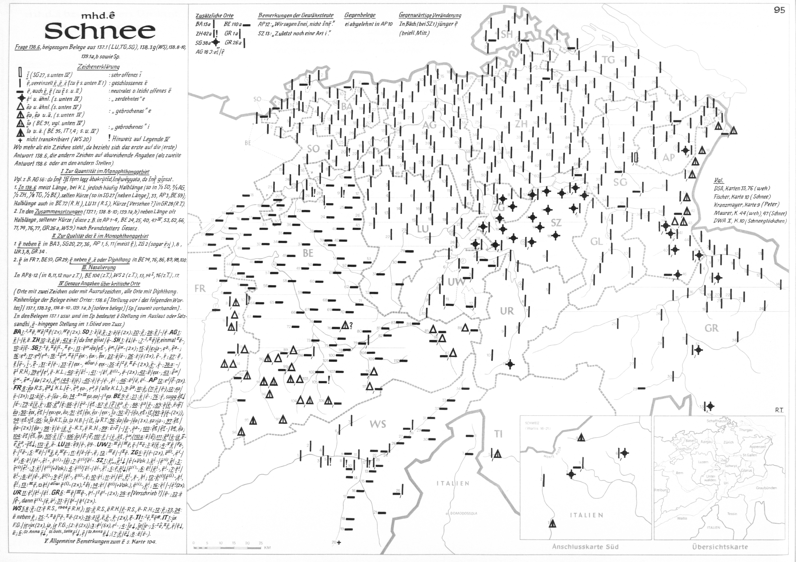
Scanned map 1/095 "Schnee" (SDS).
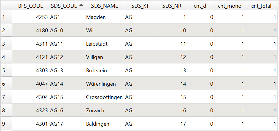
Attribute table filled during digitization of SDS map 1/095.
In contrast to other dialect atlases (e.g. of the Romance tradition), where complete transcriptions of words are written on the map, the original SDS maps are symbol maps, where each symbol represents a specific variant. Different cartographic symbols (symbol forms, hatching, colors) are used to represent different aspects of a linguistic form. We separated these different aspects by dividing one original map into several working maps (cf. footnote 1 for an example). Furthermore, we adopted a few simplification steps to speed up the digitization process: phonetically similar variants were grouped together, variants attested in less than five inquiry points were discarded, and the eight inquiry points located in Northern Italy were removed altogether.
The digital data tables can be visualized as point maps in a straightforward way (see DEFAULT). In an additional step, the point maps were converted into probabilistic surface maps by interpolation (Rumpf et al. 2009) in light of their use for machine translation and dialect identification purposes.
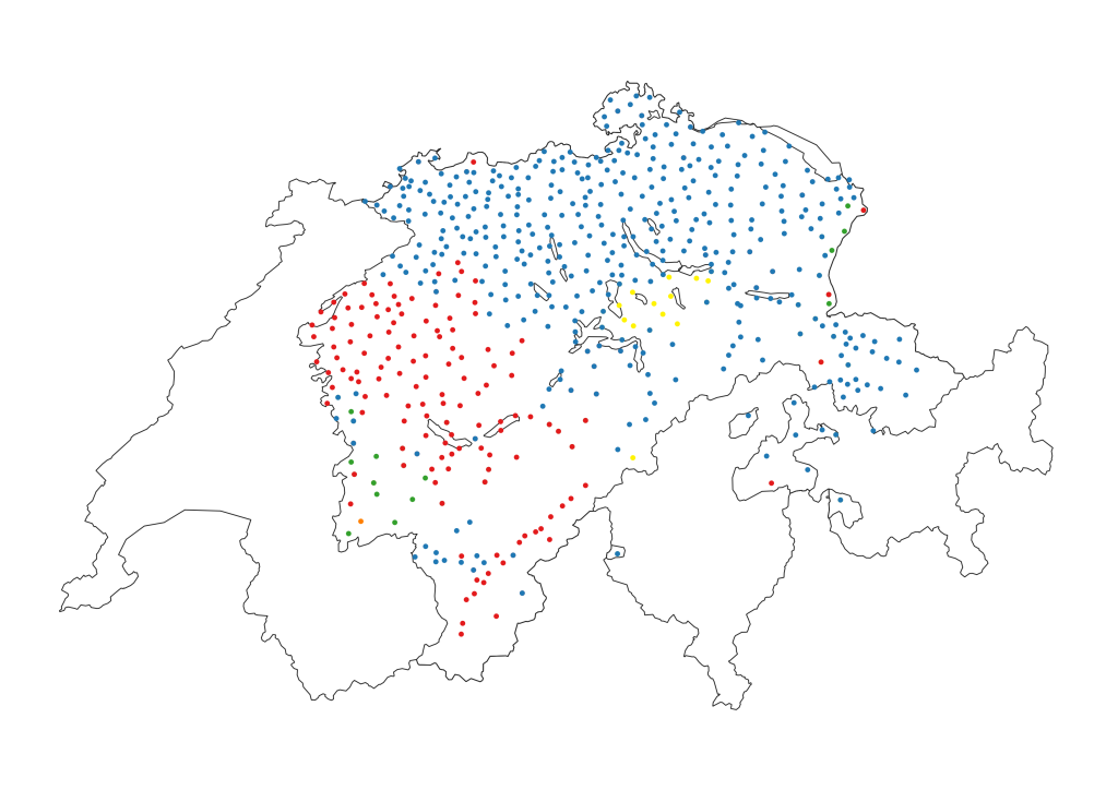
Digitized version of SDS map 1/095 "Schnee". Each point represents an SDS inquiry point, and each color represents a distinct pronunciation variant. The web-based interactive visualization of the same map is presented in DEFAULT.
This work was made available to the public by means of an interactive visualization web site. This site contained both point maps and interpolated surface maps, as well as demonstrators of the machine translation and dialect identification applications. The visualizations made use of the Google Maps rendering engine, which at the time was the most functional mapping toolkit available. Scherrer 2010 describes the contents of this web site in more detail. A few years later, the domain name <www.dialektkarten.ch> was introduced to provide an easier access to the web site.
Between 2011 and 2014, first steps were taken towards the quantitative analysis of the digitized material using the dialectometrical toolbox (Goebl et al. 2013, Scherrer 2014). The results of these studies were also integrated into the visualization web site. In the context of a Master’s thesis at the University of Zurich, further experiments were carried out. These involved additional digitized SDS maps as well as syntax data extracted from the SADS project (Kellerhals 2014). In 2014, an additional set of SDS maps was digitized at the University of Zurich, and in 2016, updated dialectometrical analyses were published as Scherrer/Stoeckle 2016.
Figure shows the distribution of digitized SDS maps over time. As explained above, there is no one-to-one relationship between atlas maps (i.e. scans) and working maps: an original map may contain several independent features that are best represented as distinct working maps,1 and several original maps may need to be combined to create a single working map with complete coverage.
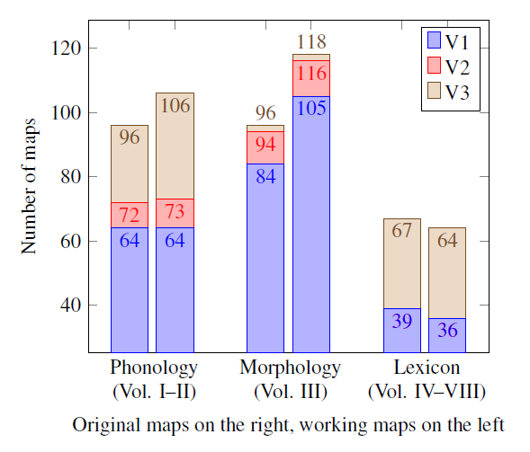
Statistics of digitized SDS maps. The V1 maps were digitized by Scherrer (University of Geneva), the V2 maps by Kellerhals (University of Zurich) and the V3 maps by Weiss (University of Zurich).
For lack of time, the visualization web site was not updated with the latest data, and development activity was reduced to essential maintenance work. In July 2018, the visualizations became unusable due to a change of the terms of service of Google Maps. This prompted us to reconsider the technological choices made eight years earlier and to move entirely to open source technologies. This move required a comprehensive rewrite of the entire web site, which was carried out over the course of 2019 and is described in detail in Section .
3. Dialectometry in Salzburg
In his seminal work, Goebl 1984 lay the foundations of dialectometry and applied the methods to digitized material from the Linguistic Atlas of Italy and Southern Switzerland (Sprach-und Sachatlas Italiens und der Südschweiz) (Jaberg/Jud (eds.) 1928-1940, henceforth AIS) and the Atlas Linguistique de la France (Gilliéron/Edmont (eds.) 1902-1910, henceforth ALF). Over the years, the methodology was refined and the data basis increased by digitizing further maps of the two atlases (Goebl 2000, Goebl 2008). In the 1990s and 2000s, dialectometrical analyses were proposed for additional dialect atlases: Goebl/Schiltz 1997 proposes an analysis of British English based on the Survey of English Dialects (SED); Goebl 2003 analyzes the Linguistic Atlas of Dolomitic Ladinian and neighbouring dialects (ALD-I) (ALD-II); Goebl 2013a reports on the dialectometrization of the Linguistic Atlas of the Iberic Peninsula (ALPI); Goebl 2013b describes similar work on the Linguistic Atlas of Catalan (ALDC).
The dialectometrical computations and visualizations were carried out using a purpose-built application for Windows systems, named Visual DialectoMetry (VDM, Goebl 2004). However, it became increasingly evident that such a stand-alone application would not permit satisfactory dissemination of the obtained results. Besides static maps of selected results, the web site <www.dialectometry.com> also showcased an interactive visualization tool based on a Java applet by Slawomir Sobota. Unfortunately, this tool stopped working around 2015 when the major web browsers ended their support for Java applets.
The upcoming rewrite of the Swiss German visualization tool provided a good opportunity to design it as generically as possible, such that additional linguistic areas and additional visualization types could be included easily. Further details of this integration will be given in the next section. Currently, the French (using ALF data), Italian (using AIS data), British English (using SED data), Iberic (using ALPI data) and Catalan (using ALDC data) linguistic areas are represented on the web site. Table shows some basic statistics of the underlying data sets.
| Atlas | Working maps | Digitized original maps | Coverage of atlas maps |
|---|---|---|---|
| AIS | 3911 | 1705 | 100% |
| ALF | 1681 | 626 | 40% |
| SED | 1524 | Extracted from various sources, all based on the raw material of SED: Atlas of English sounds (AES), Computer-developed linguistic atlas of England (CLAE), Linguistic atlas of England (LAE), Word geography of England (WGE) | |
| ALPI | 375 | 62 | 83% |
| ALDC | 1660 | 788 | 4 of 9 volumes |
4. Description of the visualization web site
The current version of the web site supports the interactive visualization of digitized working maps and dialectometric result maps.2 The maps are drawn with the Leaflet mapping toolkit, using Stamen terrain maps as backgrounds. These backgrounds are based on OpenStreetMap data. All these libraries and sources are licensed under Creative Commons or other open source licenses.
4.1. Digitized working maps
Figure shows a screenshot of a Swiss German point map. The map itself takes up most of the screen, whereas the rightmost part is reserved for user interaction (e.g. to select a different map) and metadata display (e.g. legends and information about processing). Each color represents a different variant, and variants are ordered by decreasing frequency. Gray points without letter represent SDS inquiry points in which none of the listed variants is used, either because of genuine lack of data in the original SDS data, or because of the removal of low-frequency variants during the digitization process.
Note that a point symbol may hide another one beneath it wherever multiple answers are listed in the SDS for a single location. Hidden points can be uncovered by gradually unchecking the most frequent variants in the list. Furthermore, as shown in Figure , by clicking on a point symbol, the municipality name and identification code is displayed.
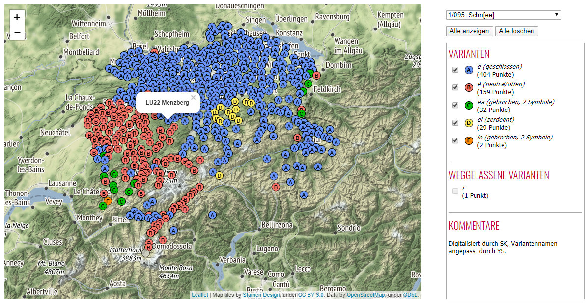
Interactive visualization of SDS map 1/095 "Schnee" as a point map (direct link). Each color represents a different variant, as shown in the legend on the right side.
Technically, the point map visualizations rely on three data files:3
- A GeoJSON file containing the coordinates and names of all SDS inquiry points. An excerpt of this file is given below:
{"type": "FeatureCollection", "features": [
{"geometry": {"type": "Point", "coordinates": [7.81309, 47.52703]}, "type": "Feature", "id": "AG1", "properties": {"name": "Magden"}},
{"geometry": {"type": "Point", "coordinates": [7.84519, 47.5575]}, "type": "Feature", "id": "AG2", "properties": {"name": "Möhlin"}},
...
]} - A JSON file listing the available maps together with their variants and other metadata:
[
{"fileid": "1095_Schnee", "title": "1/095: Schn[ee]", "variants": [
{"id": "e_geschl", "name": "e (geschlossen)", "nbpoints": 404, "color": "#6b98ff"},
{"id": "e_neutr", "name": "è (neutral/offen)", "nbpoints": 159, "color": "#ff776b"},
{"id": "ea", "name": "ea (gebrochen, 2 Symbole)", "nbpoints": 32, "color": "#01bf00"},
{"id": "ei", "name": "ei (zerdehnt)", "nbpoints": 29, "color": "#ffed5c"},
{"id": "ie", "name": "ie (gebrochen, 2 Symbole)", "nbpoints": 2, "color": "#fd8d08"}
], "comments": ["Digitalisiert durch SK, Variantennamen angepasst durch YS."], "discarded": ["i [1]"]},
...
] - A JSON file that associates, for a selected map, the inquiry points with the variants:
{

    "e_geschl": ["AG1", "AG3", ...], "e_neutr": ["AG1", "AG2", ...], "ei": ["AP12", "GR6", ...], "ea": ["BE76", "BE85", ...], "ie": ["BE91", "BE95"]

}
All these files are stored statically on the server. The Leaflet mapping toolkit makes it easy to add the GeoJSON file as an additional layer on top of the map background, and to define the style (e.g. the color) of the features defined therein.
As an alternative visualization to point maps, interpolated surface maps are also available. Surface maps provide a more suggestive visual impression of the general map structure at the expense of detail. Figure shows the same linguistic feature as above in the surface map format. The interpolation uses kernel density estimation, as implemented in the Geoling toolkit. The files produced by Geoling are stored as PNG files on the server and are merely overlaid on top of the map background. The metadata of the interpolation process is transmitted to the browser as a single static JSON file.
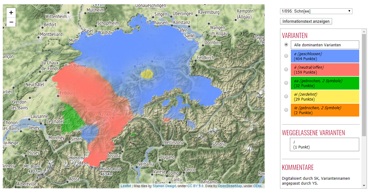
Interactive visualization of SDS map 1/095 "Schnee" as a surface map (direct link). Note the disappearance of green and red areas in the Rhine Valley (North East) in comparison with DEFAULT.
For the datasets originating in Salzburg, the visualization of working maps is currently not available. While technically simple, two main factors prevent their addition. First, the documentation concerning the taxation process and the adopted transcription system would have to be included. Second, the map search and selection tools would have to be improved: while the usability of a simple drop-down list is sufficient for the 300 SDS working maps, it would fail for the ALF or AIS projects whose number of working maps is up to an order of magnitude higher. An improved search tool should also allow users to identify maps with similar structural properties, e.g. maps with the same polynymy (Goebl/Smečka 2016).
4.2. Dialectometry maps
The general layout of the dialectometric visualization pages (e.g. the Swiss German one) is similar, with the actual map on the left and the user interaction elements on the right (see figs. , and below). Additionally, the type of visualization can be selected from the horizontal bar above the map, which currently contains six options: similarity maps, parameter maps, correlation maps, cluster maps, isogloss maps, and beam maps.
The core idea of dialectometry is to obtain abstract representations of dialect landscapes from large numbers of maps. Following Goebl (e.g. Goebl 2010, 438), the traditional dialectometric pipeline consists of four main steps (see DEFAULT).
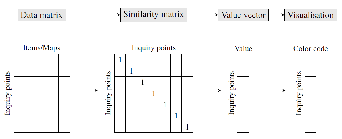
The dialectometrical pipeline.
The first step consists in aggregating information of several maps into a data matrix, such that it contains one row for each inquiry point and one column for each working map. The cells represent the variants that are used in a given inquiry point for a given linguistic phenomenon. Data matrices may cover all (digitized) maps of an atlas, or subsets thereof defined by levels of linguistic analysis (e.g. phonology or morphology).
In the second step, the data matrix is transformed into a square similarity matrix with as many rows and columns as there are inquiry points. For each pair of inquiry points, a similarity value is computed by comparing the two corresponding rows of the data matrix. Several similarity measures have been proposed, such as Relative Identity Value (RIW) or Weighted Identity Value (GIW) (Goebl 2010, 439).4
In the third step, the similarity matrix is evaluated. In other words, each row of the similarity matrix is summarized by a single value that is then visualized in a suitable way. The values are stored in a value vector. Different visualizations are based on different types of “summaries”:
- Similarity maps relative to a selected inquiry point are created by simply selecting one column from the similarity matrix.
- Statistical parameter maps are created by computing a statistical parameter (such as maximum, mean, standard deviation) over each row of the similarity matrix.
- Cluster maps are created by applying a hierarchical clustering algorithm to the similarity matrix; the resulting values represent the class of membership of each row.
- Correlation maps are based on two similarity matrices of the same shape. The map is created by computing the correlation coefficient for each pair of rows.
- Isogloss maps and beam maps represent connections between adjacent points on the map. Their value vector thus contains more rows than the similarity matrix (namely, as many as they are pairs of adjacent inquiry points) and is populated by looking up specific cells in the similarity matrix.
Other dimensionality reduction algorithms such as multidimensional scaling or principal component analysis have also been used in the context of dialectometry. These algorithms are currently not supported.
The value vector, which contains continuous (i.e., quantitative) values (except for cluster maps), could be projected directly onto a continuous range of colors. However, findings in the field of quantitative thematic cartography show that maps that are easier to grasp by the human eye if they use a small number of distinct colors (e.g. six). Therefore, a fourth step is added to the pipeline, which groups the continuous values of the value vector into a small set of color classes. Again, various options are available.
As a result of this pipeline, each inquiry point (or pair of inquiry points for isogloss and beam maps) is associated with a color class. In our visualizations, the inquiry points are represented by colored Thiessen/Voronoi/Haag polygons. Isogloss maps are based on polygon edges, whose color and thickness represent the linguistic difference between adjacent inquiry points. Beam maps rely on Delauney triangles, i.e. lines that link adjacent inquiry points; their color and thickness represent strength of linguistic similarity. Figures , and present example visualizations.
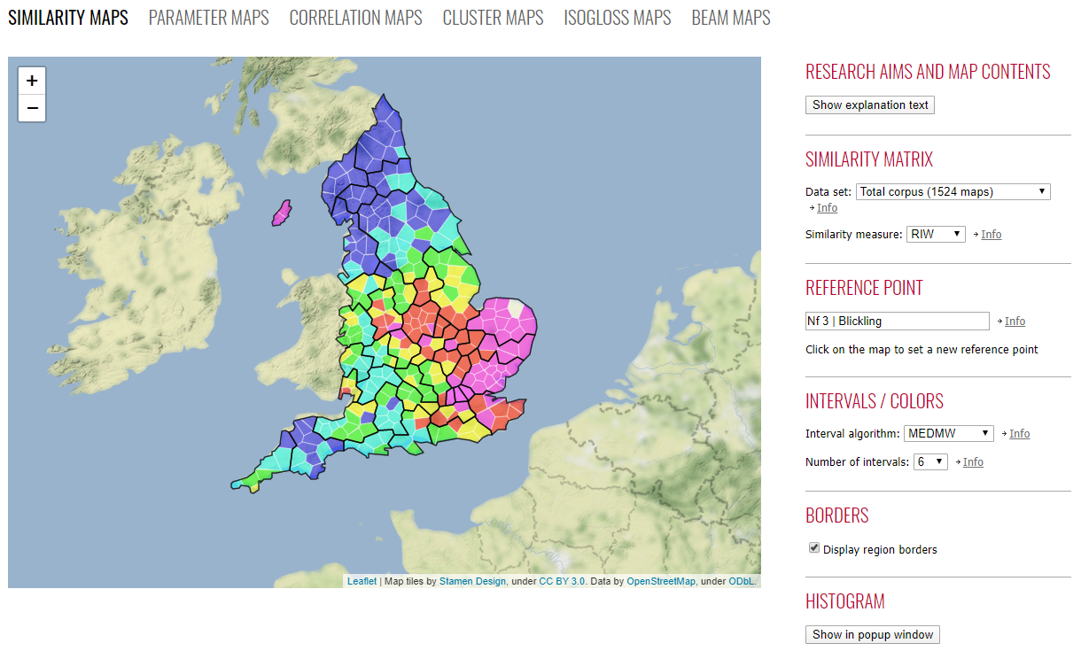
Similarity map of the British English dialect landscape (direct link). The colors depict linguistic similarity with respect to the white polygon (Blickling in Norfolk): high similarity in warm colors and low similarity in cold colors.
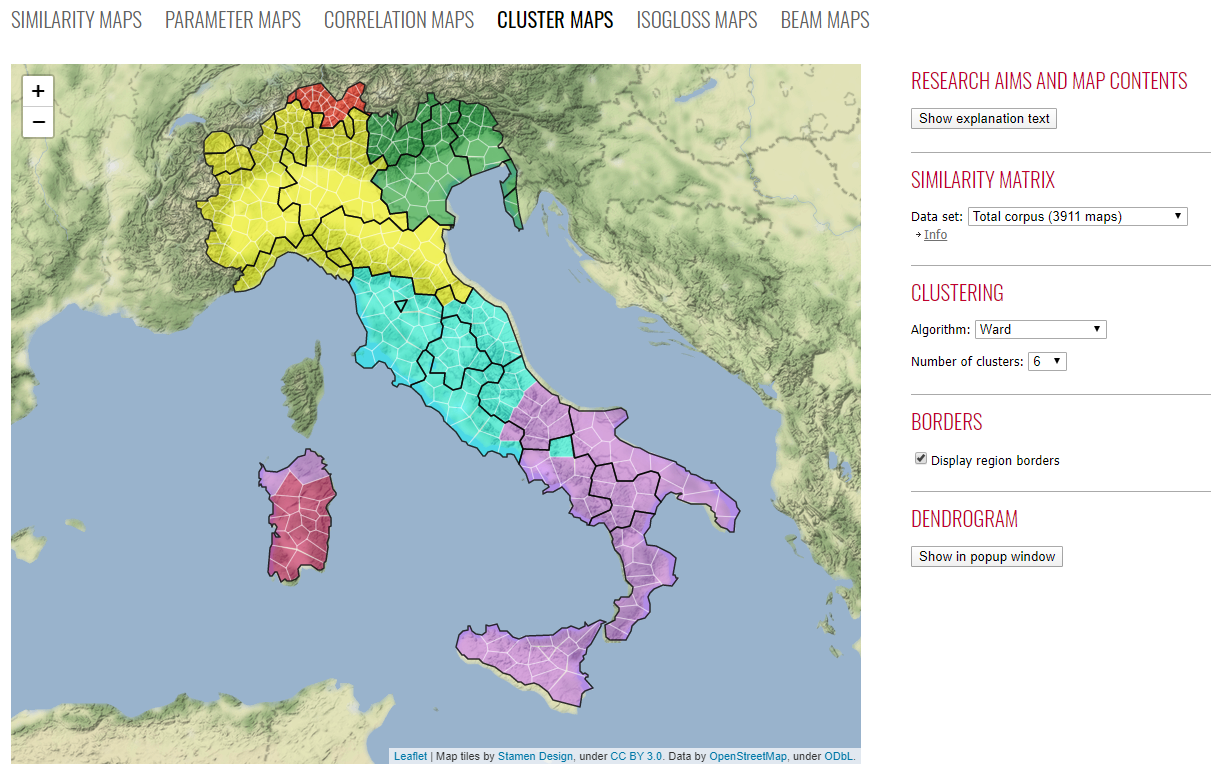
Cluster map of the Italian dialect landscape (direct link). As shown on the right, the clustering is created with the Ward algorithm and displays 6 clusters.
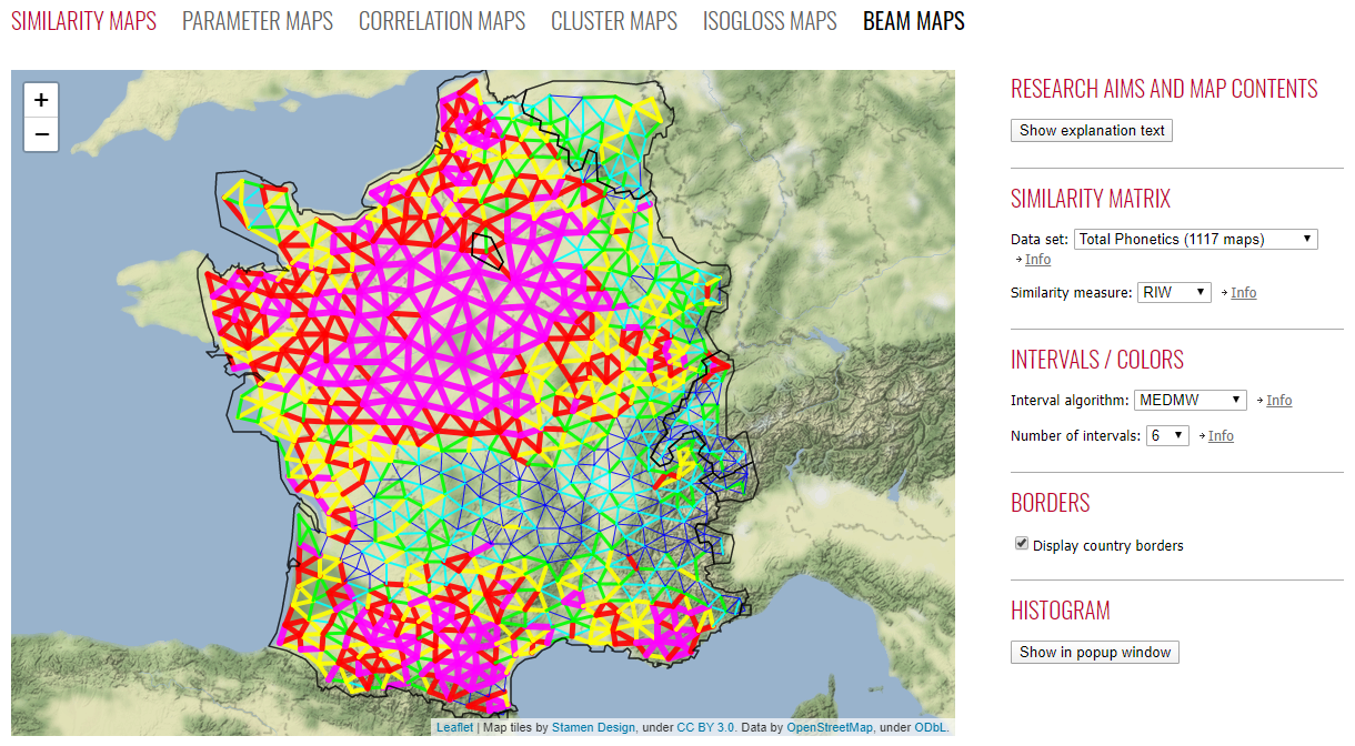
Beam map for the French dialect landscape (direct link). Each beam connects two adjacent inquiry points. The color and thickness of a beam depicts the level of similarity between the two points it connects. As shown on the right, this visualization is based only on the "Phonetics" subset.
Each visualization is thus characterized by a set of options that parameterize the four steps of the pipeline. These options can be easily modified on the right side of the map. Every change of option will immediately trigger the regeneration of the corresponding map.
The entire dialectometry pipeline is implemented in VDM, but unfortunately VDM cannot be connected directly to a web server. There are two main strategies for bringing the dialectometrical results to a web application. In the first strategy, all computations are done within VDM, for all possible combinations of parameters, and the resulting color class files are stored statically on the web server. This approach has the drawback of yielding a large number of files and is limited by the functionalities of VDM. The second strategy is to rely as little as possible on VDM and to implement the dialectometrical pipeline entirely on the web server, so that the color classes can be generated on-the-fly from the data matrices. This approach limits the storage requirements, but involves a lot of computations, which potentially slows down the responsiveness of the site.
We opted for an intermediate approach: only the first step of the dialectometrical pipeline is performed with VDM. The resulting similarity matrices are stored on the server. The remaining steps have been re-implemented as Python scripts and are carried out dynamically on the web server. This provides, in our view, a good compromise between flexibility and responsiveness. An exception is made for cluster maps: since hierarchical clustering is computationally more expensive, the cluster definition files are precomputed with VDM.
The communication between server and client is – again – based on JSON and GeoJSON files5:
- A GeoJSON file containing the coordinates and names of all polygons (or lines). The identifiers correspond to the VDM-internal numbering:
{
"type": "FeatureCollection", "features": [
{"geometry": {"type": "Polygon", "coordinates": [[[7.832, 47.541], [7.797, 47.558], ...]]}, "type": "Feature", "id": "1", "properties": {"name": "AG1 | Magden"}},
...]
} - A JSON file that defines, for a given visualization type, the colors and values to be associated with each polygon (or line):
{
"1": {"color": "#0000ff", "class": 0, "value": 42.7},
"3": {"color": "#0000ff", "class": 0, "value": 45.3},
"4": {"color": "#0000ff", "class": 0, "value": 35.2},
}
The color classification algorithm produces a particular frequency distribution of inquiry points, depending on the number of chosen color classes. The corresponding histogram can be displayed in a popup window by clicking on the corresponding button. Figure shows an example of this functionality. Hierarchical cluster analysis produces a tree, which is then cut at a predefined place to create distinct clusters. The underlying tree (“dendrogram”) can be visualized in the same way, as exemplified in Figure . The histogram and dendrogram visualizations rely on the D3 library.
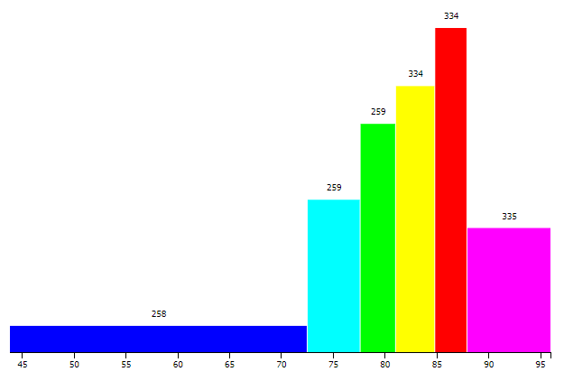
Histogram corresponding to the beam map shown in DEFAULT.
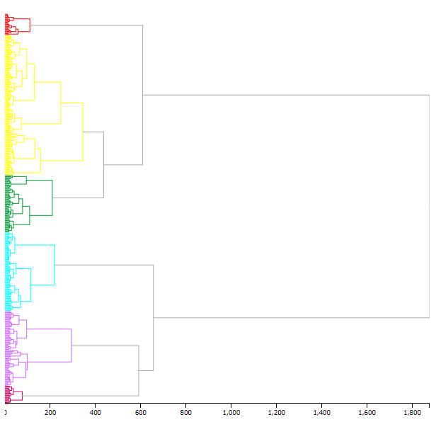
Dendrogram corresponding to the cluster map shown in DEFAULT.
Finally, it should be highlighted that the visualization web site is available in two languages (German and English) for the Swiss German part and in four languages (German, English, French and Italian) for the AIS, ALF and SED parts. Spanish and Catalan versions are available for some atlases as well. Furthermore, all options and choices in the interface are complemented with “Information” links. When clicked, they open a popup window that documents and explains the option in detail.
5. Conclusion
This paper provides a short presentation of <www.dialektkarten.ch>, an interactive web site that provides visualizations of dialectological atlases and dialectometrical analyses. The foundations of this web site have been laid in 2010, and it has been continuously expanded over the years. Major extensions have seen the light since 2019:
- The mapping engine has been changed from Google Maps to Leaflet.
- The architecture of the site has been rearranged to account for various “projects”.
- Besides Swiss German, additional projects based on digitized material from the Salzburg dialectometry group have been added. These projects currently cover data from the ALF, the AIS, SED, ALDC and ALPI.
- Correlation maps, not initially present on the web site, were added.
- All documentation was updated and made available in four languages.
6. Acknowledgements
I would like to thank Hans Goebl, who kindly provided the raw material for the visualization, but also contributed to the development of the visualization tool with numerous suggestions and bug reports. The information pages and the multilingual localization of the web site are also mostly his work.
I would also like to thank the University of Helsinki for hosting the <www.dialektkarten.ch> web site.
Bibliography
- AIS = Jaberg, Karl / Jud, Jakob (Hrsgg.) (1928-1940): Sprach- und Sachatlas Italiens und der Südschweiz (AIS), vol. 8, Zofingen, Ringier .
- ALD-I = Goebl, Hans / Bauer, Roland / Haimerl, Edgar (Hrsgg.) (1998): Atlant linguistich dl ladin dolomitich y di dialec vejins, 1a pert / Atlante linguistico del ladino dolomitico e dei dialetti limitrofi, 1a parte / Sprachatlas des Dolomitenladinischen und angrenzender Dialekte, 1. Teil, vol. 7 [4 voll. mit Sprachkarten / con mappe linguistiche (vol. I: 1-216; vol. II: 217-438: vol. III: 439-660; vol. IV: 661-884), 3 voll. mit Indizes / con indici (vorwärts alphabetisch / alfabetico: X, 823 pp.; rückwärts alphabetisch / inverso: X, 833 pp.; etymologisch / etimologico: X, 177 pp.], Wiesbaden, Dr. Ludwig Reichert Verlag [3 CD-ROM (Salzburg 1999), 1 DVD (Salzburg 2002)] (Link).
- ALD-II = Goebl, Hans (2012): Atlant linguistich dl ladin dolomitich y di dialec vejins, 2a pert / Atlante linguistico del ladino dolomitico e dei dialetti limitrofi, 2a parte / Sprachatlas des Dolomitenladinischen und angrenzender Dialekte, 2. Teil, Strasbourg, Éditions de Linguistique et de Philologie (Link).
- ALDC = ALDC (1998): Atles Lingüístic del Domini Català (Link).
- ALF = Gilliéron, Jules / Edmont, Edmond (Hrsgg.) (1902-1910): Atlas linguistique de la France (ALF), vol. 10, Paris, Champion [Neudruck: Bologna, Forni, 1968] (Link).
- ALPI = García Mouton, Pilar / Fernández-Ordóñez, Inés / Heap, David / Perea, Maria Pilar / Saramago, João / Sousa, Xulio (Hrsgg.) (2016): El Atlas Lingüístico de la Peninsula Ibérica de Tomás Navarro Tomás (Link).
- Goebl 1984 = Goebl, Hans (1984): Dialektometrische Studien: Anhand italoromanischer, rätoromanischer und galloromanischer Sprachmaterialien aus AIS und ALF, Tübingen, Niemeyer [3 vol.].
- Goebl 2000 = Goebl, Hans (2000): La dialectométrisation de l'ALF: présentation des premiers résultats, in: Linguistica 40, 209-236.
- Goebl 2003 = Goebl, Hans (2003): Spitzes und Gefiedertes aus dem Ladinienatlas (ALD-I). Sechs Taxierungsbeispiele ad usum dialectometrarum, in: Bernhard, G. / Kattenbusch, D. / Stein, P. (Hrsgg.), Namen und Wörter. Freundschaftsgabe für Josef Felixberger zum 65. Geburtstag, Regensburg, 79-105.
- Goebl 2004 = Goebl, Hans (2004): VDM - Visual Dialectometry. Vorstellung eines dialektometrischen Software-Pakets auf CD-ROM (mit Beispielen zu ALF und Dees 1980), in: Narr (Hrsg.), Romanistik und neue Medien. Romanistisches Kolloquium XVI, Tübingen, 209-241.
- Goebl 2008 = Goebl, Hans (2008): La dialettometrizzazione integrale dell'AIS. Presentazione dei primi risultati, in: Revue de linguistique romane 72, 25-113.
- Goebl 2010 = Goebl, Hans (2010): Dialectometry and quantitative mapping, in: Lameli, Alfred / Kehrein, Roland / Rabanus, Stefan (Hrsgg.), Handbücher der Sprach- und Kommunikationswissenschaft [HSK], vol. 2, 30, Berlin, De Gruyter, 433-457, 2201-2212.
- Goebl 2013a = Goebl, Hans (2013): La dialectometrización del ALPI: rápida presentación de los resultados, in: Herrero, E. Casanova / Rigual, C. Calvo (Hrsgg.), Actas del XXVI Congreso Internacional de Lingüística y de Filología Románicas (Valencia 2010), vol. 4, Berlin, Boston, 143-154.
- Goebl 2013b = Goebl, Hans (2013): La dialectometrització dels quatre primers volums de l'ALDC, in: Estudis Romànics 35, 87-116.
- Goebl et al. 2013 = Goebl, Hans / Scherrer, Yves / Smečka, Pavel (2013): Kurzbericht über die Dialektometrisierung des Gesamtnetzes des „Sprachatlasses der deutschen Schweiz“ (SDS), in: Schneider-Wiejowski, B. / Haselhuber, J. (Hrsgg.), Vielfalt, Variation und Stellung der deutschen Sprache, Berlin, Boston, De Gruyter Mouton, 153-176 [ID: unige:30844] (Link).
- Goebl/Schiltz 1997 = Goebl, Hans / Schiltz, Guillaume (1997): A Dialectometrical Compilation of CLAE 1 and CLAE 2. Isoglosses and Dialect Integration, in: Viereck, W. / Ramisch, H. / Händler, H. / Marx, C. (Hrsgg.), The Computer Developed Linguistic Atlas of England 2, Tübingen, 23-32.
- Goebl/Smečka 2016 = Goebl, Hans / Smečka, Pavel (2016): The Quantitative Nature of Working Maps (WM) and Taxatorial Areas (TA): A Brief Look at two Basic Units of Salzburg Dialectometry (S-DM), in: Kelih, E. / Knight, Róisín / Mačutek, Ján / Wilson, Andrew (Hrsgg.), Studies in Quantitative Linguistics, vol. 23, Lüdenscheid, RAM-Verlag, 113-127.
- Kellerhals 2014 = Kellerhals, Sandra (2014): Dialektometrische Analyse und Visualisierung von schweizerdeutschen Dialekten auf verschiedenen linguistischen Ebenen, Zürich, University of Zurich [MSc thesis].
- Rumpf et al. 2009 = Rumpf, Jonas / Pickl, Simon / Elspaß, Stephan / König, Werner / Schmidt, Volker (2009): Structural Analysis of Dialect Maps Using Methods from Spatial Statistics, in: Zeitschrift für Dialektologie und Linguistik, vol. 76, 3, 280-308.
- Scherrer 2010 = Scherrer, Yves (2010): Des cartes dialectologiques numérisées pour le TALN, in: Actes de la 17e conférence sur le Traitement Automatique des Langues Naturelles (TALN 2010), Montreal.
- Scherrer 2011 = Scherrer, Yves (2011): Morphology Generation for Swiss German Dialects, in: Mahlow, Cerstin / Piotrowski, Michael (Hrsgg.), Communications in Computer and Information Science 100, Berlin, Springer, 130-140.
- Scherrer 2014 = Scherrer, Yves (2014): Computerlinguistische Experimente für die schweizerdeutsche Dialektlandschaft: Maschinelle Übersetzung und Dialektometrie, in: Huck, Dominique (Hrsg.), Zeitschrift für Dialektologie und Linguistik, Beihefte 155, Stuttgart, Steiner, 261-278.
- Scherrer/Stoeckle 2016 = Scherrer, Yves / Stoeckle, Philipp (2016): A quantitative approach to Swiss German-dialectometric analyses and comparisons of linguistic levels, in: Dialectologia et Geolinguistica, vol. 24, 1, De Gruyter, 92-125.
- SDS = Hotzenköcherle, Rudolf / Schläpfer, Robert / Trüb, Rudolf / Zinsli, Paul (Hrsgg.) (1962-1997): Sprachatlas der deutschen Schweiz, Bern, Francke.
- SED = Orton, Harold / Halliday, Wilfrid J. / Dieth, Eugen / Wakelin, Martyn F. (Hrsgg.) (1962-1971): Survey of English Dialects, The Basic Material, Leeds, E.J. Arnold.